

Updated October 2026
A stress strain curve is a graphical representation of how a material deforms under loading, with stress plotted against strain. Its initial slope describes stiffness; later features may show yielding, maximum stress in tension and fracture. See what test conditions and axis labels say first, because a graph of one material or one test method may be defined differently.
This guide follows an engineering stress-strain curve from a uniaxial tensile test, with familiar landmarks of a ductile metal. Worked numbers are assumed for teaching. Composites, polymers and compression tests require their own definitions; curves may not always follow the same order.
Stress Strain Curve: Axes and Units
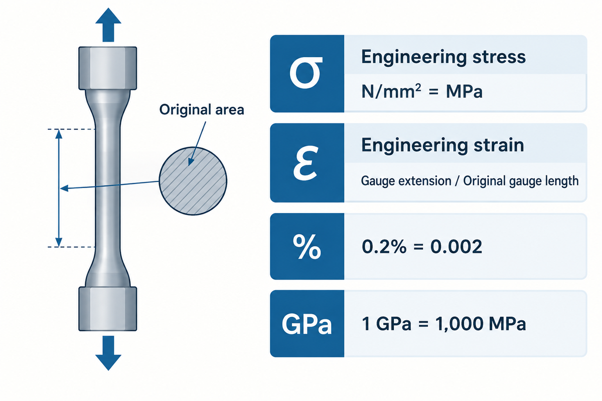
Engineering stress is force divided by original area. Engineering strain is change in gauge length divided by original gauge length. A stress axis in MPa and a strain axis in percent describe different quantities. Read the axis labels before comparing slopes: a percentage axis changes the numerical slope by a factor of 100.
For a specimen loaded in the axial direction, write stress as σ = F/A0 and strain as ε = ΔL/L0. Stress is defined as force per unit area. Strain is dimensionless when both lengths are given in the same unit. The University of Illinois material-behavior reference gives engineering definitions and the relationship between stress and strain for these material behaviors.
| Quantity | Calculation or unit | Reading rule |
|---|---|---|
| Engineering stress | N/mm² = MPa | Use the original cross-sectional area. |
| Engineering strain | mm/mm | Use extension within the original gauge length. |
| Percent strain | 100 × decimal strain | A plotted 0.2% means ε = 0.002. |
| Elastic modulus | MPa or GPa | 1 GPa = 1,000 MPa; divide by decimal strain. |
What is the difference between elongation and strain?
Elongation is a change in length, such as extension measured in millimeters. Engineering strain divides the change in length by the original length. With this normalization, specimens with different gauge lengths may be compared. Percent elongation also needs its measurement convention. Extension during loading and permanent elongation after fracture are two different results.
A supplier spreadsheet headed “extension” should define a length unit and a gauge length field. Without the required definitions, conversion of x-axis to engineering strain isn’t reliable. Keep the original force and elongation channels alongside the calculated curve. They help to discover unit mistakes. The curve represents their normalized relation, not an independent, second measurement.
Elastic Region and Modulus of Elasticity
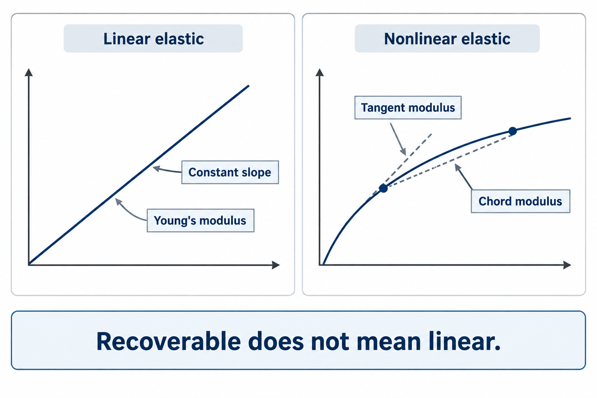
In the initial stage, the elastic region behaves like a spring. When stress is applied and removed, the specimen returns to its original shape. A linear section shows a constant slope, which is defined as Young’s modulus. Steeper lines indicate higher stiffness under comparable conditions; a University of Illinois table lists 210 GPa for mild steel, 2 GPa for plastic. Yield strength is a separate property, read later, for example where the 0.2% offset line meets the curve.
To determine the modulus of elasticity for the initial linear portion, use the formula E = Δσ/Δε, where Δε is expressed in decimal strain. A two-point calculation demonstrates the principle, but a laboratory modulus result requires the specified fitting method, strain interval and instrument accuracy. Avoid fitting across seat movement, slip or curved transitions into yielding.
What is the relationship between stress, strain and Young’s modulus?
Stress is related to strain by Young’s modulus in the linear elastic range. When the curve becomes nonlinear, one constant slope no longer describes the entire response. A local slope is described by a tangent modulus, and a slope over a stated interval is described by a chord modulus. Report the definition and test mode used.
ASTM E111-17(2025)e1 separates Young’s, tangent, and chord moduli. Its public scope excludes the initial-tangent and secant modulus determinations. It states the tensile and compressive moduli may be different. “Elastic” means that a response is recoverable, and therefore an elastic response may be curved. “Linear” means that the relationship has a constant slope.
“Precise determination of Young’s modulus requires due regard for the numerous variables that can affect such determinations.”
ASTM E111-17(2025)e1, public Significance and Use, section 5.5
At small strains, choice of measurement may become critical. A strain gauge built into a load cell is part of the force measurement chain; crosshead displacement may include grip movement and machine deformation. An appropriate contact or optical extensometer would measure the specimen extension.
“the displacement of the crosshead may not represent the actual elongation of the test sample, rendering the calculations incorrect.”
For an incoming inspection report, ask which displacement channel supplied strain, and which points were entered in the slope fit. A machine-generated modulus column may look exacting, but may use an inappropriate displacement channel.
Yield Strength and the 0.2% Offset
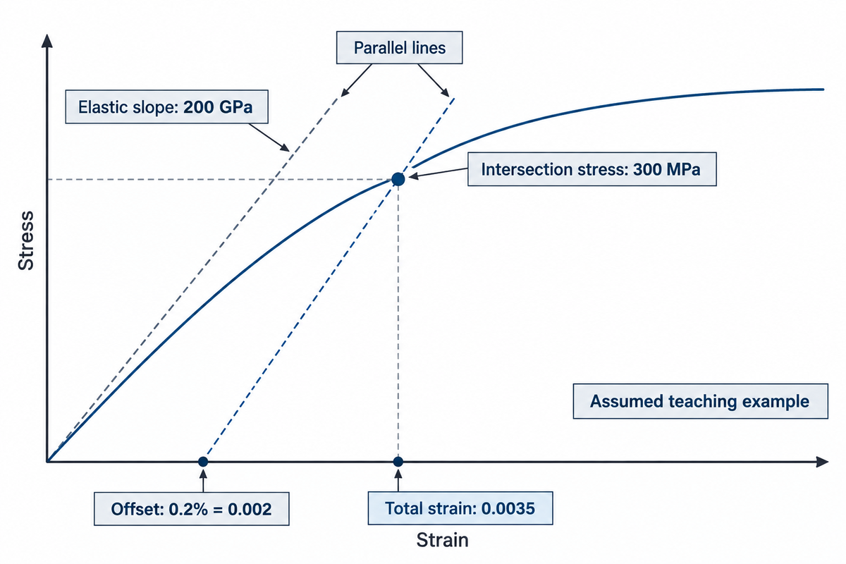
A 0.2% offset line starts from decimal strain 0.002, and is parallel to the elastic line. Its point of intersection with the measured engineering curve gives the prescribed offset yield strength. The total strain at that point of intersection includes the elastic contribution and the prescribed offset.
Certain metals exhibit a yield point; others, a gradual transition into the plastic region. Michigan Tech’s tensile-test explanation describes an offset method to locate the yield stress where the transition isn’t sharp. Use the offset described in the pertinent material specification, rather than presuming all tests use the same value.
For an assumed elastic modulus of 200 GPa, the offset line is σ = 200,000(ε − 0.002) MPa. Suppose that line intersects an assumed test curve at total strain 0.0035. The stress value is then 200,000 × (0.0035 − 0.002) = 300 MPa. The total strain is 0.35%, although the offset remains 0.2%.
This construction represents the yield strength according to the chosen proof criterion. It doesn’t locate the first irreversible microscopic event. Once plastic deformation occurs, unloading along an elastic return path leaves residual extension: the material is permanently changed in length. A purchase requirement should define the proof or yield definition, so that the two reported values mean the same thing.
Ultimate Tensile Strength, Necking and Fracture
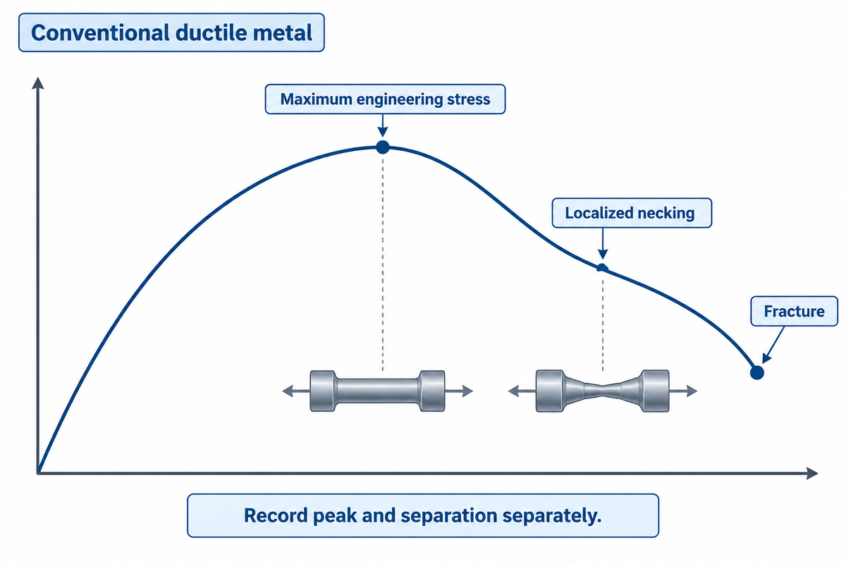
Ultimate tensile strength (UTS) represents the maximum engineering stress reached during the tensile test: maximum load divided by original area. On a conventional ductile-metal curve, the peak is commonly followed by localized necking and then fracture. The fracture point is the point at which the material separates, so the engineering stress can be less than the peak value.
Before the peak, strain hardening can allow the specimen to carry increasing load while it deforms plastically. Metal plasticity comprises dislocation motion; the detailed hardening response depends on the material and its condition. As a neck develops, deformation concentrates in a smaller region instead of being uniform across the gauge length.
Engineering stress is defined as the supported load divided by the original area. After the peak, the supported load starts to decrease and the same trend is shown by the engineering stress curve. This shows a real change in the defined force-to-area quantity. However, this alone does not identify the change in local flow resistance of the material inside the neck.
Record the peak load and the load at separation separately. A report that names the final point “ultimate strength” requires clarification before using the tensile strength of the material for comparisons. Fracture elongation and reduction of area describe ductility in different ways; neither replaces the strength value.
Engineering vs True Stress-Strain Curves
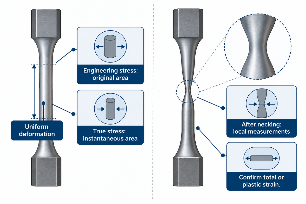
Engineering stress is calculated using the original area; true stress uses instantaneous area. True strain accumulates incremental extension relative to the changing length. With a suitable approximation of uniform deformation, engineering data can be converted to true stress-strain curves. Once necking localizes deformation, the same global conversion no longer gives a dependable local flow curve.
For the uniform deformation approximation, σtrue = σeng(1 + εeng) and εtrue = ln (1 + εeng) . David Roylance’s stress–strain notes at MIT restrict this approximation to the beginning of necking. In the relevant regime of deformation, this approximation holds, and volume constancy is an assumption.
After localization, average extension in gauge doesn’t imply strain is uniform everywhere in the specimen. Estimating local true stress using current area also requires care, as a multiaxial stress state develops during necking. A constitutive model calibrated for simulation may require local geometry and strain measurements as well as appropriate corrections or inverse analysis.
MetalForming’s discussion of digital image correlation demonstrates how, in the region of necking, local optical measurements extend strain observations. The article also indicates that determining stress may be complicated. A conversion in a spreadsheet alone is insufficient.
When a simulation supplier asks for a “true curve,” determine whether the input is total strain or plastic strain, what stress measure is needed, and where the calibrated data end. Extending the last measured segment by eye modifies the model; it doesn’t add a measurement.
Ductile and Brittle Curves Across Materials
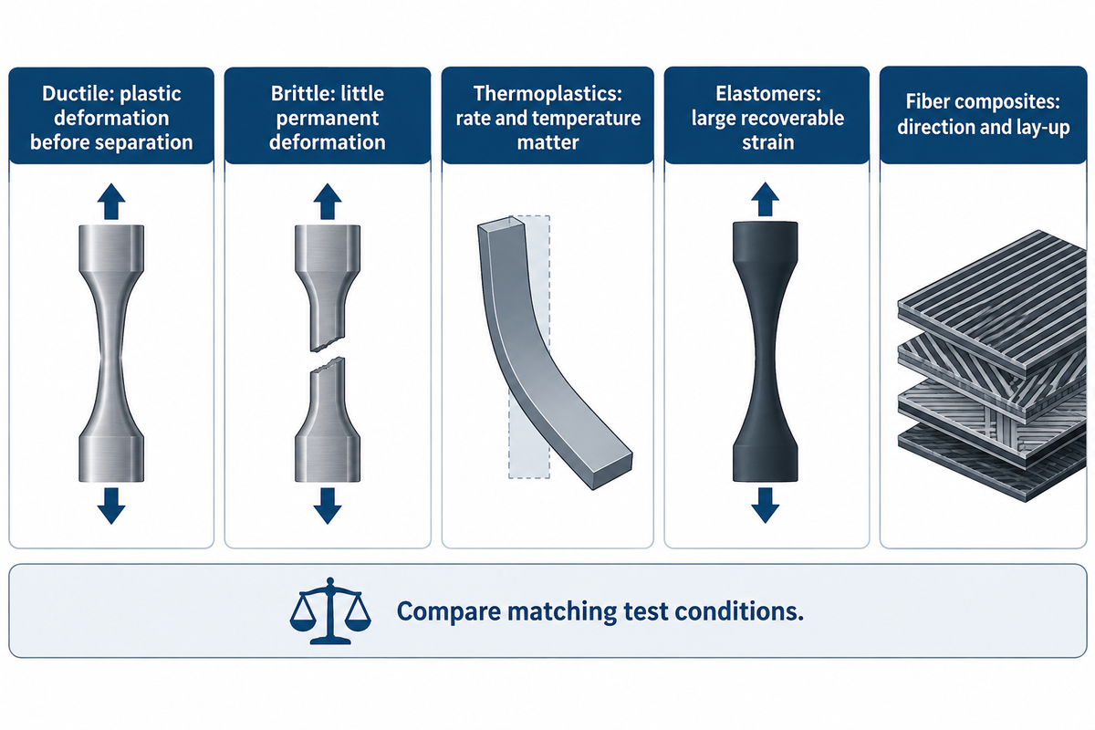
A ductile material shows significant plastic deformation before separation, while brittle materials may fracture with little permanent deformation in the test conditions used. Different materials therefore produce different curve shapes. A familiar metal diagram is a good start, but yield plateaus, necking and a distinct linear stage aren’t universal features.
These mechanical properties are case specific. Changes in shape should be analyzed in the context of similar test conditions. Cold working or heat treating a metal modifies its behavior; the same is true for anisotropic materials, where orientation is important. The curve of a material belongs to a particular case and specimen direction, not to a general term, such as a metal, non-metal or plastic.
Nonlinear response with temperature and loading rate sensitivity is observed in some thermoplastics. Elastomers can exhibit a large amount of strain and recover almost completely. A fiber composite requires the loading direction and lay-up to be identified. Use the appropriate polymer or composite test method when interpreting the reported strength and strain.
Compression adds its own complications. Contact friction and specimen barreling can affect a compressive test. Select tensile or compressive results for the stress mode of interest. A tensile-only test curve isn’t automatically suited for a compression model.
To compare machining, begin with the actual part condition in the drawing and material order. Our pages on ABS material behavior and fiberglass properties provide material specific information. The test report requires its own specimen and methodology.
Toughness and Modulus of Resilience
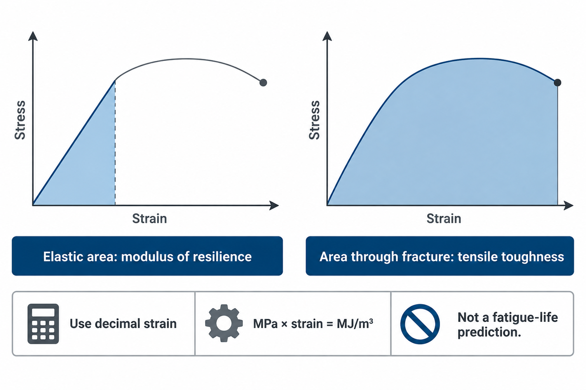
The area under an engineering stress–strain curve measures tensile work per original specimen volume. The elastic portion of the result gives the modulus of resilience; the area through fracture gives a measure of tensile toughness for that test. A steep curve that fractures at low strain can enclose less area, and so less tensile toughness, than a lower curve that stretches further.
What is the area under the curve of a stress-strain graph?
Stress integration with respect to strain results in energy per unit volume for the loading case defined. For a linear elastic segment, the triangular area is one-half stress times strain. During integration, use decimal strain; values presented in percent need to be converted. Integrating percent strain without conversion results in an overstated energy density by a factor of one hundred.
With stress in MPa and strain being dimensionless, the unit of integration is MJ/m³. It measures tensile work per original volume, which differs from fracture toughness defined in the context of crack growth. The full curve area alone does not provide a prediction of fatigue life.
According to strength of materials, the loading convention determines the meaning of an energy calculation. The report needs to state which endpoint and measure of strain were used in the integration. If an extensometer was removed prior to separation, check how the remaining extension was measured, and then compare total areas.
Curve Analysis: A Worked Reading Example
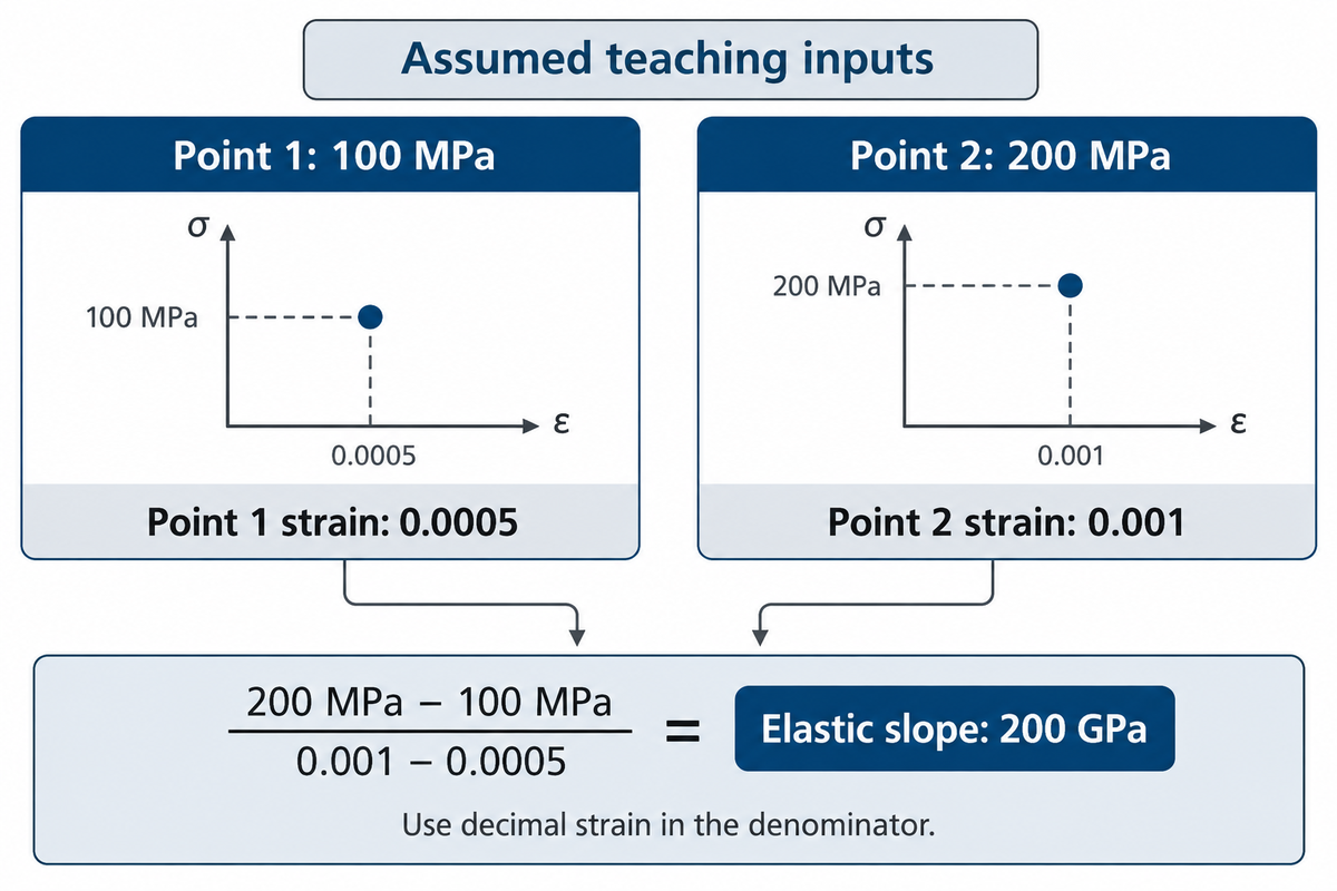
In curve analysis, measured channels and original dimensions are converted to the quantities reflected on the graph. The example presented here assumes a uniform specimen and a linear elastic segment. This illustrates handling units and the calculation of slope, and isn’t a representation of a measured dataset for a specific alloy.
4-Point Curve Reading Map
Read four landmarks in sequence: initial elastic slope, specified yield or proof point, maximum engineering stress, and fracture. Check axes before the first landmark and method of measurement before comparing any two curves. The example gives the elastic calculation; locating the other landmarks requires the rest of the measured curve.
| Check | Assumed input or calculation | Decision it supports |
|---|---|---|
| Original area | A₀ = 50 mm² | Use the same original area for both engineering stresses. |
| Original gauge length | L₀ = 50 mm | Normalize the measured gauge extension. |
| First applied force | F₁ = 5,000 N | Keep the raw load channel. |
| First extension | ΔL₁ = 0.025 mm | Use specimen extension, not uncorrected machine travel. |
| First stress | 5,000 N ÷ 50 mm² = 100 MPa | Convert force into engineering stress. |
| First strain | 0.025 mm ÷ 50 mm = 0.0005 = 0.05% | Check decimal and percent columns. |
| Second applied force | F₂ = 10,000 N | Use a second point inside the same linear range. |
| Second extension | ΔL₂ = 0.050 mm | Check the original gauge length has not changed in the denominator. |
| Second stress and strain | 200 MPa; 0.001 = 0.10% | Do not divide stress by the printed percent value. |
| Elastic slope | (200 − 100) MPa ÷ (0.001 − 0.0005) = 200,000 MPa = 200 GPa | Arithmetic result for the assumed elastic segment. |
The formulas follow the definitions used in materials science; the inputs are deliberately chosen for a transparent calculation. A laboratory would select the interval and fitting procedure required by its method rather than infer a certified modulus from two convenient points.
For a receiving inspection, an unexpected slope is a reason to check the channels before rejecting a batch. For an engineering design, a correct slope leaves the strength, fatigue, and service loading to be evaluated. A simulation handoff requires the original data as well as the transformed data, so that the next engineer checking the handoff can evaluate the conversion.
Stress-Strain Data: Sources and Tensile Testing Costs
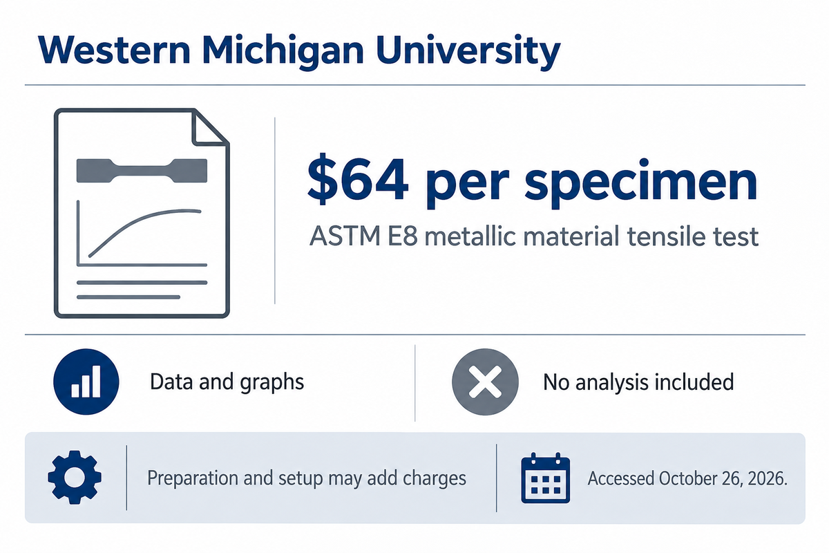
Western Michigan University’s public schedule lists an ASTM E8 metallic material tensile test at $64 per specimen (accessed October 26, 2026). That example has a dataset and graphs with no analysis. Preparation and other work can add charges, so compare the measurements and delivery requirements prior to comparing laboratory rates.
The Bronco Construction Research Center fee schedule lists additional charges for machining, sample preparation, fixturing and significant setup at applicable hourly and material rates. Preparation is billed at staff rates of $20.00 to $72.84 per hour, so request a total estimate after the laboratory has assessed the samples. Its posted line item doesn’t define every strain channel or reporting option. Confirm these in the test quote request.
For a specific condition, e.g. alloy and heat treatment, start with the producer’s data for that condition. For comparison, refer to a materials handbook or published research curves. For acceptance of purchased stock, have the appropriate lot-specific test records and lot traceability evaluated. For engineering design, obtain the approved allowables or model data required by the application.
ASTM E8/E8M-25 is the active metallic tension-test edition listed by ASTM at this review. Its public scope defines room temperature as 10–38°C unless otherwise specified. It generally uses 4D and 5D gauge lengths for round specimens under the respective unit-system methods, with stated exceptions. Record the actual geometry instead of treating E8 and E8M as labels that can be swapped.
A request for a particular test should include the material condition and specimen orientation, the method and revision, temperature, strain-rate control, sensor arrangement, required results and raw-data format. Indicate if the lab has to prepare the specimens and if extension through fracture is required. This scope prevents a simple load-only test from being misinterpreted as a modulus and strain test.
An Eng-Tips discussion of irregular tensile curves provides an excellent example of a practical report-review prompt. Before interpreting an irregular tensile curve, check that measurement channels are functioning, and review software fitting options. The discussion provided several possible explanations, including slip in the grip or extensometer; these aren’t verified diagnoses. A plotted label is a starting point for an investigation.
Curve Selection for CNC Material Decisions
Choose a curve based on the condition of the material, mode of loading and intended use consistent with the case before you. A representative curve from the datasheet is useful to compare candidates; traceable lot tests address acceptance criteria. Structural-integrity work needs a third record: the approved design allowables or calibrated model data the application requires.
| Record or curve type | Useful for | Check before use |
|---|---|---|
| Engineering tensile curve | Comparing tensile response in the tested condition | Original dimensions, material condition and strain measurement. |
| Force–displacement record | Reviewing machine channels and specimen response | Whether displacement is crosshead travel or gauge extension. |
| True curve before necking | Uniform-deformation material modeling | Conversion assumptions and total versus plastic strain. |
| Post-necking local curve | Studying localized deformation | Local geometry, strain measurement and stress-state treatment. |
| Typical supplier datasheet | Early material screening | Grade, heat treatment, direction and statistical basis. |
| Lot-specific tensile report | Checking agreed purchase acceptance criteria | Lot identity, sampling plan, method and required limits. |
| Nonlinear elastic curve | Modeling recoverable nonlinear response | Tangent/chord definition and operating strain interval. |
| Compression curve | Evaluating compressive response | Test geometry, friction, barreling and mode-specific properties. |
| Simulation input table | Running the chosen constitutive model | Units, stress/strain measures, calibration range and extrapolation. |
The selection matrix incorporates university definitions and cautions from ASTM about specimen and test scope. This is a working review aid to help design, quality and procurement teams; it does not set material acceptance limits. Define acceptance limits on the applicable drawings, specs or purchase orders.
Strength data require manufacturing context. Check the machinability comparison to narrow material options. A hardness result can address an indentation issue. However, it shouldn’t be used to make up an entire stress–strain curve for an unknown case.
Do
- Match the material condition and specimen direction.
- Keep the raw force and gauge-extension channels.
- State the property definition in the purchase requirement.
Don’t
- Read percent strain as decimal strain.
- Label fracture stress as the peak automatically.
- Extend a global conversion through necking without justification.
For a part that’s to be machined, consider Zhenling Metal’s CNC material options, along with the drawing and the required condition of the material. Send the preferred grade, heat treatment and acceptance requirements of the component to discuss the material and the scope of machining together.
Discuss Your Material and Drawing Requirements
FAQ
What is the formula for calculating strain as a percentage?
Engineering strain as a percentage is 100 times the change in gauge length divided by the original gauge length.
Use matching length units in the numerator and denominator. Keep decimal strain in calculations for elastic slope or energy density, even if the graph displays percent. The report should also state whether extension was measured during loading or after fracture, because recovered elastic extension changes the meaning of the final elongation value.
What does necking look like on a stress-strain curve?
Necking is localized thinning; in a conventional ductile-metal engineering tensile curve it commonly develops around the maximum-load region.
The falling branch after the peak reflects decreasing force divided by the unchanged original area. Local deformation can continue while this engineering stress falls. To identify what is happening within the narrowed region, inspect the specimen and suitable local measurements; the global curve alone does not reveal the complete local stress state.
How does temperature change a stress-strain curve?
Temperature can change the slope and the rest of the curve, not always in one direction: in tests on high-strength structural steels, strain at fracture fell up to about 400 to 500 °C, then rose above room-temperature values.
Compare curves at the temperature relevant to the application rather than applying a universal correction. Loading rate, thermal history and material condition should also match. A room-temperature result is a defined laboratory condition, not a measurement across the full service-temperature range. Request tests or validated data covering the temperature range used in the design.
Are stress-strain curves always linear?
No. Stress-strain curves are linear only up to the proportional limit, where stress and strain stay proportional; above it, a curve can turn nonlinear while still elastic.
Many materials depart from that relationship. Nonlinear elastic deformation can recover on unloading, whereas plastic deformation leaves a permanent change. Look at unloading behavior and the applicable material model before assigning a label.
How do I plot a stress-strain curve in Excel?
Use an XY scatter chart with calculated strain on the horizontal axis and calculated stress on the vertical axis.
Place the original force and gauge-extension data in separate columns. Divide force by original area to calculate engineering stress, then divide extension by original gauge length to calculate engineering strain. Check the force and length units before plotting. Use decimal strain for calculations and format the axis as percent only when appropriate. Preserve the raw columns and note the gauge length, specimen area and sensor. A line chart with equally spaced categories can hide unequal strain intervals, so choose numerical XY axes.
When is Hooke’s law valid on the curve?
Hooke’s law holds on the initial part of the curve, up to the proportional limit, where deformation is linear and elastic.
Beyond that interval, a single constant modulus cannot describe increasing strain accurately. Identify the fitted range and avoid extending the straight line into plastic deformation or assuming it captures nonlinear elastic behavior.
How can I compare two stress-strain curves fairly?
Compare curves with matching stress and strain definitions, material conditions and test methods before comparing their landmarks.
Start with the units and whether the strain axis is decimal or percent. Check grade, heat treatment, orientation, temperature, loading rate and specimen geometry. Then confirm how strain was measured and which yield or proof definition was used. A typical curve and a lot-specific result answer different questions, even if the labels name the same alloy. If the reports differ in method or scope, resolve those differences before ranking stiffness, strength or ductility. Keep acceptance criteria separate from a visual preference for one curve.
Connecting Material Data to a Machining Inquiry
Zhenling Metal supplies custom machined components from drawings or samples. This guide explains how stress–strain terminology connects material selection with a clear purchasing requirement. The calculation uses assumed teaching inputs; the laboratory price belongs to the named university. For a component inquiry, share the grade and condition together with the drawing so that tensile-property requirements are discussed as part of the material scope.
References & Sources
- Mechanics Reference: Material Behavior, University of Illinois
- Tensile Test Experiment, Michigan Technological University
- Stress-Strain Curves, David Roylance, MIT
- ASTM E111-17(2025)e1, Public scope and significance
- ASTM E8/E8M-25, Public scope and significance
- Tension and Compression Testing, Western Michigan University
- Tensile Testing: A Compressed “How-To” Overview, Quality Magazine
- Digital Image Correlation: How It Changed the Tensile Test, MetalForming